Context

We consider the fluid-structure interaction (FSI) system in which the fluid is governed by the incompressible Navier–Stokes equations in a two–dimensional domain with mixed boundary conditions, while the structure, immersed in the fluid, is modeled by the Euler–Bernoulli equations with damping, with one end clamped and the other free. The system is given by
\[\partial_t\mathbf{u} + (\mathbf{u}\cdot\nabla)\mathbf{u} - \text{div}\hspace{0.1cm}\sigma(\mathbf{u}, p) = 0, \hspace{0.2cm} \text{div}\hspace{0.1cm}\mathbf{u} = 0\hspace{0.2cm}\text{in}\hspace{0.1cm} Q_{\eta}^{\infty}:= \bigcup_{t\in(0,\infty)}\{t\}\times\Omega_{\eta(t)},\] \[\text{+ Mixed boundary condition + Initial condition + kinematic condition},\] \[\partial_t^2\eta + \alpha\Delta_s^2\eta + \gamma\Delta_s^2\eta_t = H(\mathbf{u}, p, \eta) + \textcolor{brown}{f} + f_s \hspace{0.2cm}\text{in}\hspace{0.1cm}(0,\infty)\times (0,\ell_s),\] \[\text{+ Boundary conditions + Initial condition},\] where \(\mathbf{u}\) and \(p\) represent the fluid velocity and the pressure, respectively, and \(\eta\) the displacement of the structure. Here, \(\sigma(\mathbf{u},p)\) represents the Cauchy stress tensor, \(H=H(\mathbf{u}, p, \eta)\) the force exerted by the fluid on the structure (acting on its upper and lower parts), \(\textcolor{brown}{f}\) is the control, and \(f_s\) a given constant force.

The geometrical configuration is shown in Fig. 1.

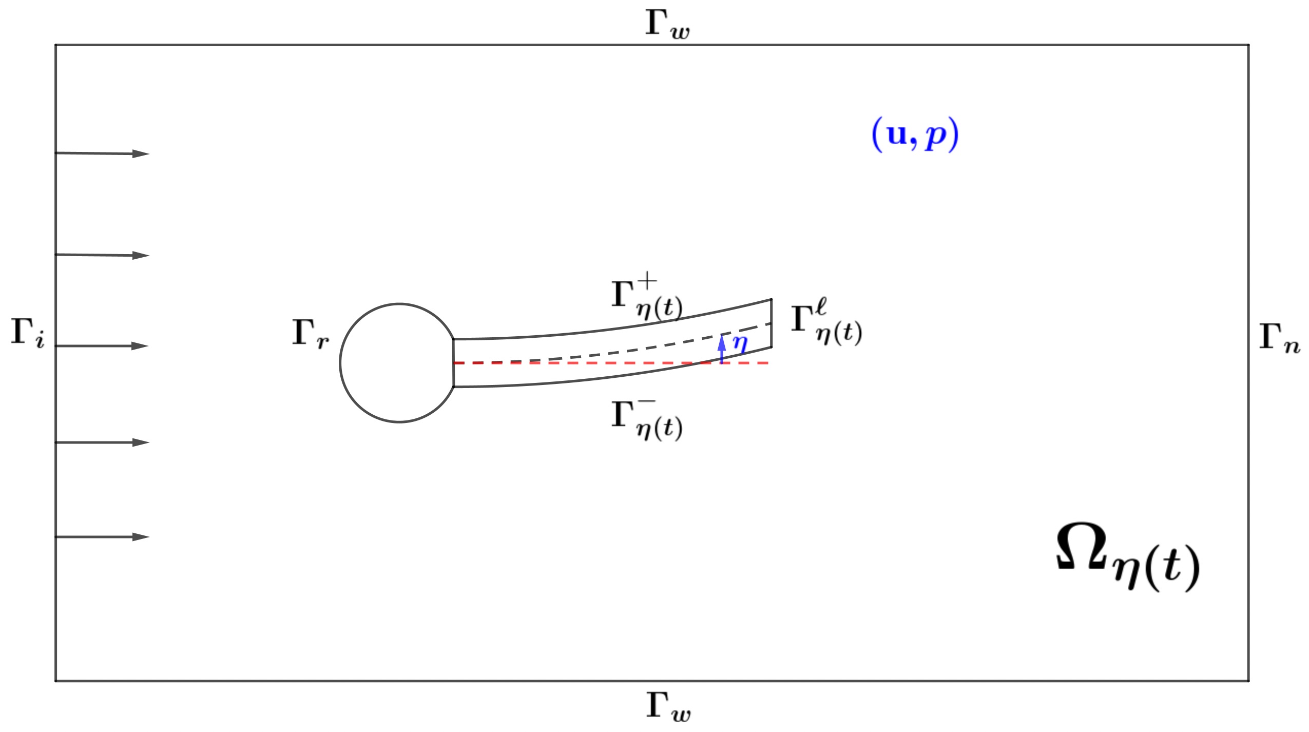
Figure 1: Physical domain.

Numerical tests

In the numerical simulations shown below, we use a Reynolds number \(Re = 200\), a rigidy coefficient \(\alpha=10^{-1}\), and a damping coefficient \(\gamma=10^{-6}\).

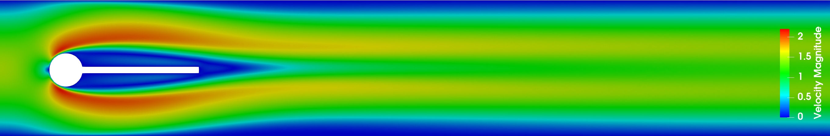
Figure 2: Magnitude of the stationary fluid velocity when \(Re=200\).

We treat the numerical implemention of the direct problem by using the Arbitrary Lagrangian-Eulerian (ALE) approach and a semi-implicit time stepping scheme. Fig. 3 shows the evolution of the mesh around the structure (without control).

Figure 3: Evolution of the mesh around the structure (without control).

To obtain the feedback law \(\mathcal{K}\) (based on the linearized system), which is assumed to be given in a feedback form, we solve a low-dimensional Riccati equation.

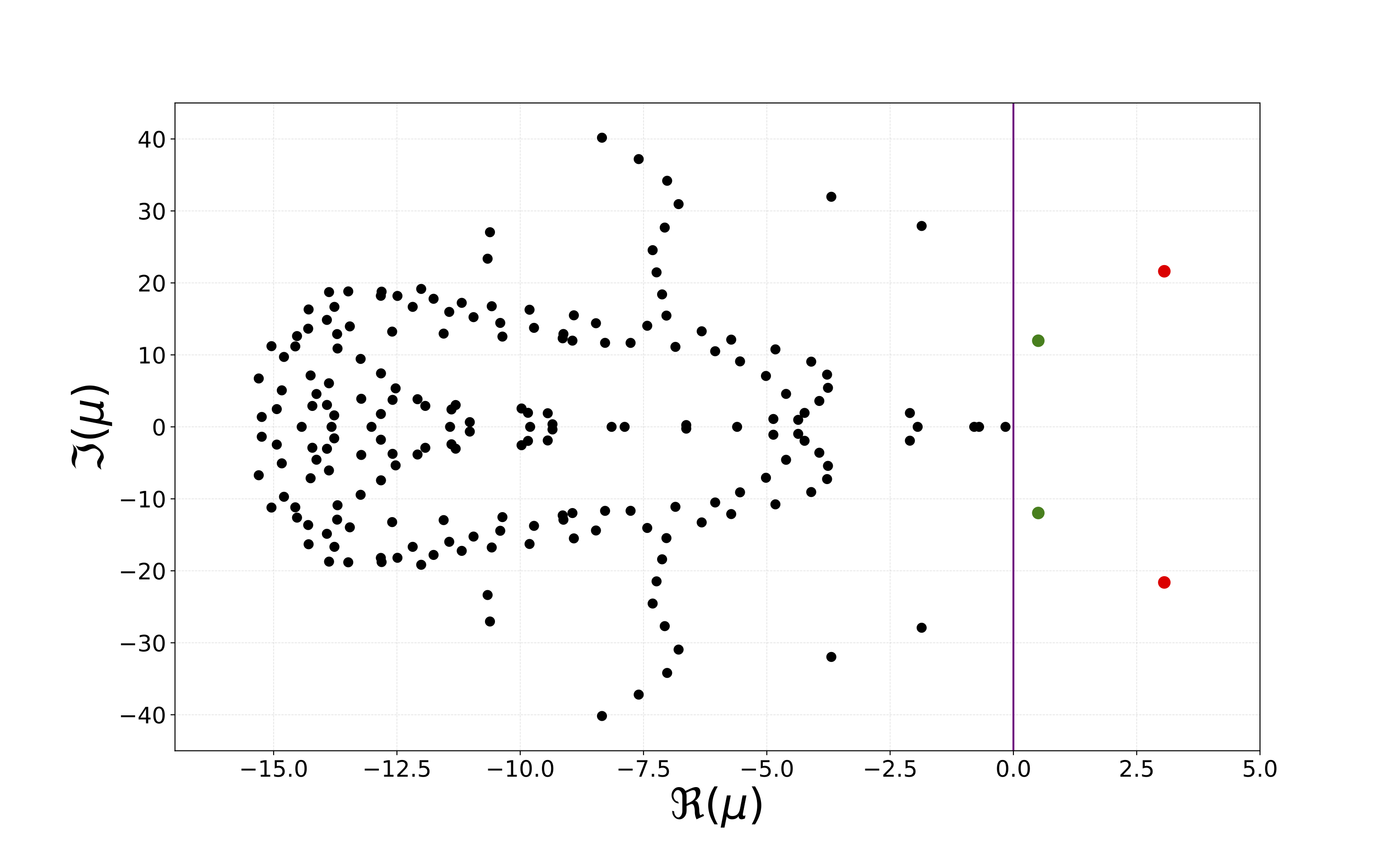
Spectrum of the FSI operator \( \mathcal{A} \).

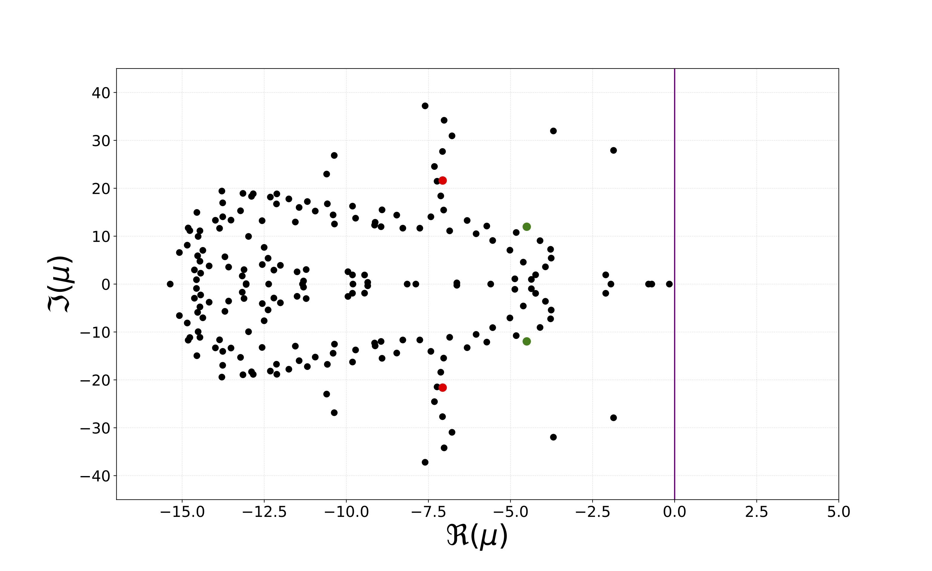
Spectrum of the operator \( \mathcal{A}-B\mathcal{K} \).

Figure 4: Comparison of the spectrum \(\sigma(\mathcal{A})\) and \(\sigma(\mathcal{A}-B\mathcal{K})\). Here, \(B\) is the control operator.

Figure 5: Fluid velocity magnitude without and with control.